Making Round Images Flat And Flat Images Round

Hi! It’s Blayze from the ShefBots Pi Wars team! Currently I’m 33,000 feet above Middle Kuyto, Finland and about two and a half hours into a 10 hour flight, so I figured now was as good a time as any to write a Pi Wars blog post!

About a month ago I posted a picture of our team’s 360-degree camera to Twitter that caught some attention:

In this post I’ll be going over the camera system and talking about some of the trials and tribulations it took to get it to work.

The Why

A number of the Pi Wars challenges require some kind of vision system in order to either pick up barrels, follow lines or go to certain areas, and in particular, the “Eco-Disaster” and “Minesweeper” challenges require quite a wide range of vision, with target objects appearing behind and in front of the robot. It seemed that these challenges the robot could benefit from being able to process it’s entire surroundings simultaneously, without the need to worry about reorienting and aligning views/measurements from a fixed-direction camera or sensor array - a process that would take up valuable in-task time and could also introduce errors into the odometry readings of the robot.

To this end I suggested that we use a 360-degree camera - namely, a camera that could take 360-degree panoramic images. The lab that I come from at the University of Sheffield studies insect-inspired robotics, and the research field is full of work that uses panoramic images to perform things like homing and positioning, providing clear evidence that the idea could work, and offering some examples to inspire design.

The Hardware

The only issue with this idea was that 360-degree cameras and lenses can be quite pricey. Fortunately, the field of biorobotics comes through for us again, with a number of robots managing to get a 360-degree field of view by using a small curved mirror above a static camera. These mirrors can be a little tricky to come by, so instead we opted for using a 20 mm diameter ball-bearing as our reflector, and a standard Raspberry Pi camera on the bottom. In total, it’s possible to build an entire 360-degree camera with an integrated computer for about 25 pounds consisting of a ball bearing, a 3D-printed housing, a Raspberry Pi Zero and a version 2.1 Pi Camera module (note that we had to go for a version 2 camera module, as this was the only module that allowed us to refocus the lens onto the ball properly. I have managed to refocus an original camera module once before, but we had a lot of issues repeating that).

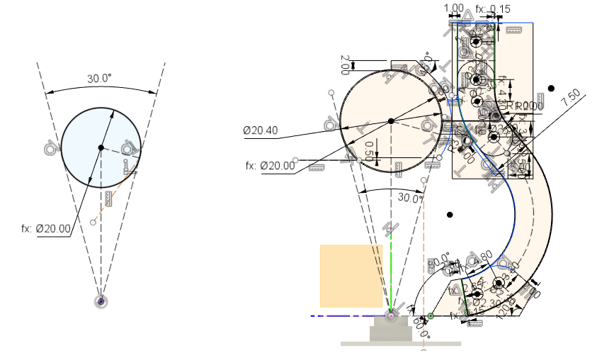
The first thing to do was to build a mount that would hold the ball bearing a reasonable distance above the camera. This went few a few versions. originally designed in OpenScad, it was quickly moved over to Fusion 360 to go along with the rest of our work (although, given it’s more open approach to CAD, I would very much like to come back and put together an OpenScad version of the final model at some point in the future). I started by positioning the camera at the origin and then set the bearing distance so that it would be exactly within the 30 degree minimum field of view of the Pi Camera (that turned out not to be the minimum field of view in practice), from here it was just a case of CAD’ing up something that’d support the bearing above the camera.

The bearing support itself went through only one major re-design. Originally I’d parametrised it such that the width and total number of supports and could be specified, which would then be placed symmetrically around the camera’s axis of view. While this was good enough for first tests, the team were concerned that the legs obscured too much of the surroundings, and they didn’t line up with the motors of the robot, which extended up into the camera’s vision anyway, so we wanted to take advantage of that and use that space to hold the supports. To that end, a second version was designed with the goal of leveraging the strength of steel to support the camera on just two support legs - although in practice, the supports were thin enough to allow for three thin 3D printer struts. The design also features A raspberry pi mount at the bottom and additional space on the top to mount a top panel to block sunlight or mount further sensors/markers.

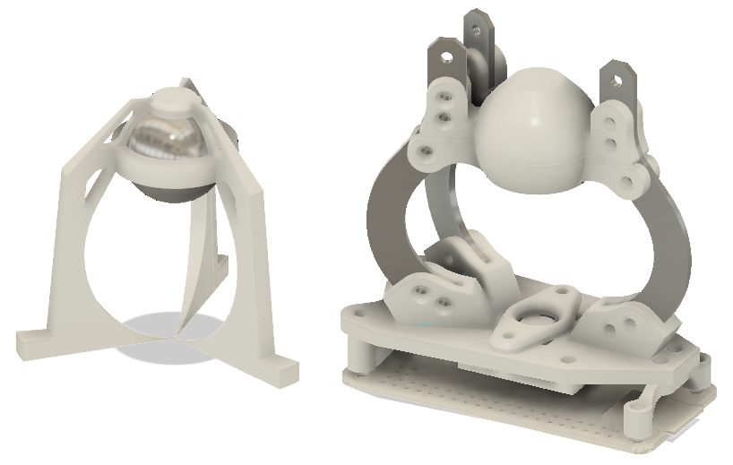
In both designs, it was very important to keep the supports as far away from the camera as reasonably possible, as closer, thicker supports would occlude more of the surroundings than thinner, further away ones - to that end both versions of the design have a sort of inverted-bulb design.

Configuring the Camera

The Raspberry Pi Camera itself can be fiddly to use in it’s own right. After discovering that my original test Pi 4 seems to have an issue transmitting or receiving large files, I switched to working entirely on the Pi Zero over USB Ethernet and wrote a few scripts to take photos with various settings altered through OpenCV in Python:

Eventually I settled on using a slightly brighter and longer exposure time that default settings to try and bring out as much colour as I could from the image. I had thought that cranking up the contrast would be a good way to pull a good colour reading from the image, but I noticed that at higher contrast settings the colours of our test barrels were being pushed down to near black, so the contrast settings were left near default. On top of this, I found the white balance to be rather temperamental, so that was left on “auto” - although I suspect that that might not be the best option, due to it potentially throwing any future processing out of whack.

Dewarping The Image

Now, up until this point I’ve only discussed practical, hands-on things that while time-consuming, aren’t exactly outside the expected when it comes to entering a challenge like Pi Wars. But now we’re about to take a detour to software engineering town, with a service-station stop at mathsville. So far, all our images have been coming in like this:

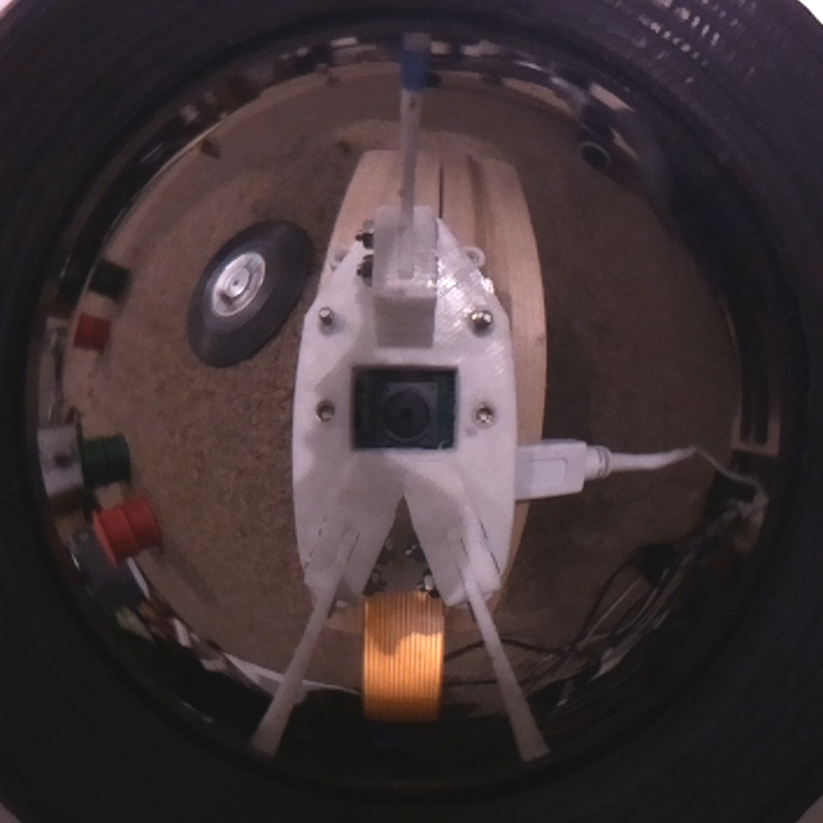
Originally the plan was to build a neural-network based solution to object recognition and assessment that would simply take these images in and tell us everything we needed to know. However, with increasing external pressures on the team’s time, we opted for a more traditional computer vision approach using OpenCV. For this we decided that dewarping the images into clean 360-degree panoramic images would make our lives much easier. We could work entirely with the raw data in polar coordinates - but that would require us to modify all of our computer vision algorithms to respect the fact that things further to the edges of the image were just warped and not actually smaller. It would also mean that we would have no idea about the angle of any given pixel from the reflector, which is incredibly useful to know when estimating distance to an object.

In order to dewarp the image, a mapping between each pixel on the output (360-degree) image and any given pixel on the input image (of a reflective sphere). The diagram below sums this up quite well:

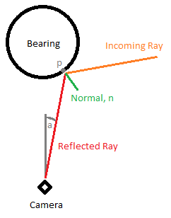
In this diagram the red line represents a ray coming from the outside world into the camera and we want to calculate the angle, a, between the incoming ray and the camera’s vertical axis. This will let us work out where in the input image we should sample a pixel from, as it is possible to simply taking the angle from the center of the image across the field of view of the camera. The ray is assumed to be perfectly reflected about the normal of the sphere (marked normal, n in the diagram), meaning that the angle between the incoming ray and n and the angle between the ray to the camera and n are equal.

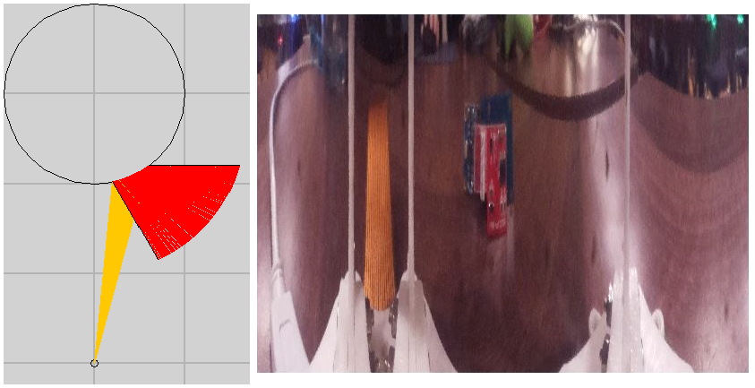
The trick is that we essentially want to work out the intersection point between the ray and the sphere (marked p in the diagram) - meaning we can intersect either the incoming line or the reflected line. Unfortunately though, lines in 2D space need both a position on the line and a gradient to describe them. On the incoming line we have no position on the line, as that is determined by the sphere’s radius, and on the reflected line we have no gradient as that is determined by it’s relationship to the incoming line. I had originally wanted to analytically solve this equation, but after a few collective hours of re-arranging and re-representing I decided that a numerical solution would be best. Similar to finding the root of an equation using numerical methods, I implemented a simulator for the system that would iterate along the length of the reflector until the reflected ray’s gradient was equal to some arbitrarily set target gradient:

This allowed a target gradient to be calculated by converting a required angle from the horizontal to a direction vector. The algorithm essentially steps every N degrees, and compares the reflected ray’s angle to the target one. If the reflected ray has passed the target, then the step angle is decreased and the direction swapped so that it goes back, this time crossing the desired angle a little closer. This continues until the target gradient is reached.

Doing this allowed me to generate angles at any given point, so all that was left was to calculate every ray gradient for every angle of a field of view (in this case, between the horizon and 60 degrees below it):

An added bonus to using a numerical approach to finding the desired angle over any analytical approach is that the solver is generalisable to non-spherical surfaces. In the future I would be interested in setting the software up so any reflective surface can be defined and an appropriate lookup table will be generated.

With every angle on the vertical generated, all that is required is some way of indicating the center of the reflector in the input image and the extent the rays can be cast to. In order to facilitate this I built an application in Java. This program displays the input image as well as a reticule, which once aligned uses the numerical method to generate a dewarping lookup table which can then be exported for use in python, allowing each pixel value of the dewarped image to be retrieved via output[x][y] = getColourAt(lookuptable[x][y][0], lookupTable[x][y][1]).

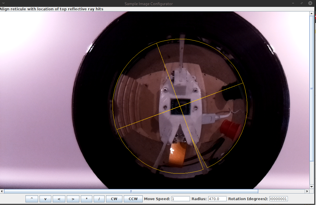
The idea behind this it that any language that can process the lookup table can dewarp the image. Indeed, the Java program itself uses the lookuptable as well as the python program running on the robot. In an ideal world this would be a very efficient task, as a lookup operation only require each pixel of the input image to be referenced via a 2D array. However, unlike in a lower-level programming language like C or C++, Python is not massively fast at looping through each and every pixel of an image, even if it’s only performing simple calculations on them (and even when the array is a numpy one!). To this end, instead of storing the dewarp table as a large 2D array and looping through x and y values of each pixel location in the output, the dewarp table is instead stored as a large single-dimensional numpy array (with one element for every pixel of the output) that stores the indices of every pixel to lookup in the input image, as if the input image were also stored in a large single-dimensional array. This means that the input image from the camera can be cast to a single-dimensional array using the numpy.resahape() command, and then the lookup table applied to it via a single output = input[dewarp] call which can then be reshaped into the correct image shape as a 2D image. This cuts the dewarping time down from 5.5 seconds to just 32 milliseconds!

The dewarper also generates an array of angles that relate to each vertical row of pixels on the dewarped image, so the angle of any given pixel’s view (relative to the downward vector) can easily be looked up, which, when paired with the height of the reflector gives a good estimate of the distance from robot to whatever piece of floor that pixel is directed toward.

In Conclusion

All in all, 360-degree field of view is almost definitely useful when it comes to robotics, but getting there can take quite a bit of work - especially if you want the image in a human-readable, deformation-free format. We’re anxious to see how this sensor performs in the field!

The dewarping software is available on GitHub - there’s already a moderately long list of upgrades that we (or, I guess, I) want to make to it to make it a more useful tool, so feel free to watch the project if you think anything mentioned here is up your alley!